What is protein aggregation?
Protein aggregation is when protein molecules stick together to form larger structures, ranging from small clusters to large complexes. It usually follows misfolding or partial unfolding, and aggregated protein commonly loses its function and may come out of solution altogether.
Why is my protein sample aggregating?
After synthesis, proteins typically fold into a particular three-dimensional conformation, the native state. That folding process can be impaired, creating misfolding or unfolding and leading to aggregate formation. In general, aggregation can be the result of various interactions, including hydrophobic, electrostatic or van der Waals forces. Proteins have hydrophobic regions that tend to interact with each other, leading to aggregation when they are exposed to an aqueous environment.
The conditions that trigger it are well known. Extremely high protein concentrations can exceed the saturation point. High temperatures can denature proteins and promote their aggregation. Changes in pH can disrupt the electrostatic interactions between proteins. Variations in salt concentration affect protein solubility. Mechanical stress, such as pipetting or vortexing, can disrupt protein structure. Freeze and thaw cycles, improper storage, exposure to light and prolonged storage or incubation all allow proteins to gradually lose stability. Contaminants or impurities in the sample can promote aggregation, and some added molecules do so directly, including detergents and denaturing agents. Mutations in the protein sequence can make a protein aggregation-prone, and post-translational or chemical modifications can alter a protein's properties and lead to aggregation. Larger proteins are more susceptible, because more surface area means more opportunity for intermolecular contact, and interactions between several proteins in the same solution can themselves produce aggregates or complexes.
Most of these are conditions under experimental control, which is why aggregation is normally studied as a function of one of them rather than measured once.
Why does aggregation matter?
Aggregation can happen naturally or under stress, and it affects both how a protein performs in an experiment and how safe a drug product is. Aggregated protein commonly loses its function, and in a binding or sizing experiment it removes material from the population you intended to measure.
It is also not only an experimental nuisance. Aggregation is central to several neurodegenerative diseases, including Alzheimer's disease, Parkinson's disease and Huntington's disease, in which particular proteins misfold and accumulate as deposits that damage neurons. Much of the interest in measuring aggregation in solution, under native conditions, follows from this. How FIDA measures amyloid fibrils and oligomers is covered in how to measure amyloid fibril length and binding in solution.
What types of aggregates are there and how do they show in FIDA data?
Aggregates are not a single population. In relation to FIDA measurements there are two categories.
Large aggregates, also called insoluble aggregates, are particles that are not undergoing diffusion. They are therefore not observed as a regular gaussian shape, but rather as individual spikes along the Taylorgram. Generally, the amplitude of the spike is related to the size of the aggregate.

Intermediate aggregates, also called soluble aggregates, are for example oligomers that are not diffusing sufficiently to satisfy Taylor's conditions. In this case the aggregates can be seen as a shoulder before the gaussian shape.

The distinction matters because the two classes appear differently in the data and are quantified differently: spikes are counted, while the soluble fraction is quantified from the fluorescent area of the larger species.
How is aggregation measured in FIDA?
FIDA measures aggregation in solution in every run, by counting large aggregates as spikes and quantifying soluble aggregates from the fluorescent area of the larger species. Aggregation is rarely a single number. It is usually measured as a function of a given parameter, such as time, different buffers or temperature, all of which can be assayed with FIDA. The quantity of interest is the trend, and the condition at which the trend changes.
FIDA captures both classes of aggregate within a single in-solution measurement, because both alter the recorded signal in ways that can be separated. Soluble aggregates contribute to the dispersion profile and can be quantified from the fluorescent area of the larger species when several populations are fitted, which gives an amount rather than a simple indication that aggregation is present.
Quantification of in-solution sample aggregation is performed ubiquitously, all throughout the measurement. Sample molecules that form large aggregates, whether big soluble or insoluble particles, often cause high light scattering and are detected as distinct spikes in the raw FIDA signal. These sample aggregates can be discretely quantified using the spike counter tool integrated in the FIDA analysis software, and each spike is at least one aggregate. As the data is loaded the number of spikes is already quantified, and with several files the counts can be tabulated, plotted and followed as the formation of spikes develops.

Where the spikes appear tells you which vial they came from
The analyte solution is used to equilibrate the capillary before injection of the indicator, and it generates the baseline signal. Spikes in the baseline signal therefore indicate aggregation in the analyte vial, and in that case the spikes are distributed throughout the total recording time frame.
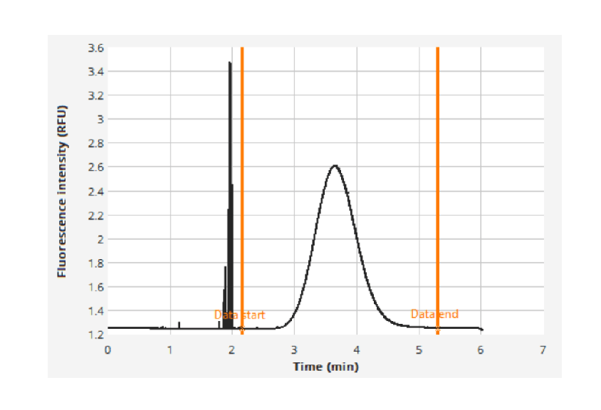
Signal spikes that appear only after the baseline signal, at the base of the gaussian peak, exclude the possibility of aggregation in the analyte vial. That time delay indicates aggregates in the indicator vial instead.
Non-diffusive aggregates larger than 1 µm in diameter typically flow along the fastest flow lane of the laminar flow, which makes them appear early in the run, predominantly before the main gaussian peak.
What the data is still worth when spikes are present
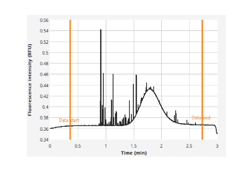
With only a few spikes the signal is noisier, but the gaussian peak can still be resolved and the size of the diffusing protein extracted. The indicator size can be measured by choosing the fitting region as the gaussian peak only, eliminating the spikes, and the Smooth Curve filter removes the spikes and analyses only the gaussian portion of the signal.
Where spikes are numerous and large enough they obscure the underlying peak entirely, and the size of the diffusing species cannot be recovered from that run. In one case there were 630 aggregates, which the spike counter reports, ruining the signal so much that the Taylorgram could not be fitted. A weak signal from the diffusive species leads to inaccurate sizing.
Because nothing is immobilised and nothing is separated, the sample is observed as it is, including in serum, plasma, lysate and formulation buffers, and aggregation is recorded alongside size and binding in the same experiment. Nanolitre volumes per data point make series against temperature, time or freeze and thaw cycles practical on limited material. Further reading: Aggregation readout.
What has FIDA shown about aggregation in real samples?
FIDA has measured aggregation in gene therapy particles, nanoparticles and stored proteins, each time in the same run as the size of the main species.
Example: FIDA counted 830 aggregates in the 40 nL used from one preparation of AAV2 gene therapy particles, against 46 in a second preparation, in the same label-free run that gave the particle size and polydispersity (360-degree automated characterisation of AAVs). FIDA followed the size of engineered Tc24 antigen variants for Chagas disease diagnostics through up to five freeze–thaw cycles and found no significant change (Batra et al., 2025). FIDA also measured the size, polydispersity and aggregation of lipid nanoparticles in buffer and in serum and plasma (Characterising lipid nanoparticles with FIDA).
What do I do if my sample is aggregating?
When FIDA shows aggregation, what to do depends on where the aggregates come from, which FIDA shows by where the spikes appear in the run.
If you observe the aggregation from the indicator alone, spin the sample down, remove the supernatant, re-evaluate the sample concentration from the supernatant and rerun the experiment. Measuring protein concentration after centrifugation matters, because the correct concentration has to be used in the binding or kinetics assay. This is the usual case after a first thawing cycle.
If the aggregates arrive after mixing with the analyte, they most likely arise from the interaction between indicator and analyte. The same approach applies: spin the samples down to check whether the interaction causes the aggregates, or whether the indicator is interacting with aggregates already formed in the analyte.
If the analyte is a protein, or a mixture of several proteins, centrifuge the stock solutions. If the analyte is a buffer, a buffer filtration step is recommended.
Heavy aggregation spikes on binding can be an agglutination effect, for instance a labelled target binding to a polyclonal antibody, where almost the entire indicator signal is lost to spikes. Changing the assay setup to CapMix mode shortens the interaction time between the two partners, or modulates it with different pressures, which may reduce the agglutination. In-capillary dilution during a CapDis measurement can also minimise agglutination and probe only the primary binding event.
Frequently asked questions
Can FIDA measure protein aggregation?
Yes. Flow Induced Dispersion Analysis (FIDA), developed by Fida Biosystems (Fidabio), detects and quantifies protein aggregation in every measurement, in solution and in any buffer, serum, plasma or cell lysate: large aggregates are counted as spikes in the signal, and soluble aggregates are quantified from the fluorescent area of the larger species. How the technology works is explained in What is FIDA?
How do I know how aggregated my sample is?
FIDA tells you how aggregated your sample is by giving you the number of aggregates and their size from the same run. Large aggregates are counted one by one as spikes, so the count can be expressed per volume of sample, and soluble aggregates are fitted as a separate, larger species, which gives their size and their share of the signal. For example, FIDA counted 830 aggregates in 40 nL of one AAV2 preparation, about 2.1 × 10⁷ aggregates per mL, while measuring the particle size at 8.5 nm and the polydispersity index at 0.1 (360-degree automated characterisation of AAVs).
How does FIDA quantify aggregation?
FIDA measurements automatically provide quantification of aggregation through a spike count. Sample molecules that form large aggregates often cause high light scattering and are detected as distinct spikes in the raw FIDA signal, and these can be discretely quantified using the spike counter tool integrated in the FIDA analysis software. For example, FIDA counted 830 aggregates in 40 nL of one AAV2 preparation and 46 in another (360-degree automated characterisation of AAVs).
How do you measure sample aggregation?
Aggregation is usually measured as a function of a given parameter, such as time, different buffers or temperature, all of which can be assayed with FIDA. The emergence of the different types of aggregates can then be quantified by measuring the number of spikes, which are the insoluble aggregates, and the total fluorescent area of larger species, which are the soluble ones.
What types of aggregates are there and how do they show in FIDA data?
Different types of aggregates can be observed with FIDA: soluble diffusive aggregates and insoluble non-diffusive aggregates. Soluble aggregates will register as a shoulder or bump on the Taylorgram, while insoluble aggregates will register as a signal spike. The soluble kind can be quantified by their total fluorescent area by fitting multiple species. The insoluble ones can be counted by counting the spikes, as each spike is at least one aggregate.
Can I still get a size if my sample has aggregates?
Yes, if the gaussian peak is still resolvable. Choose the fitting region as the gaussian peak only, or use the Smooth Curve filter, which removes the spikes and analyses only the gaussian portion of the signal. If the spikes are numerous and large enough to obscure the peak, the size cannot be recovered from that run.
Can FIDA check whether freeze–thaw cycles make a protein aggregate?
Yes. FIDA checks whether freeze–thaw cycles make a protein aggregate by measuring its size and aggregates after each cycle, from nanolitres per measurement. For example, FIDA showed no significant change in the size of engineered Tc24 antigens over up to five freeze–thaw cycles (Batra et al., 2025).
Can aggregation be measured directly in plasma or serum?
Yes. Nothing is immobilised and nothing is separated, so the sample is observed as it is, including in serum, plasma, lysate and formulation buffers. For example, FIDA measured the size, polydispersity and aggregation of lipid nanoparticles in serum and plasma (Characterising lipid nanoparticles with FIDA).
Related resources
The application note Protein Oligomerization: Easy and Accurate Determination in Plasma and Buffer works through a closely related case, and Assessment of Sample Quality with Every Measurement puts aggregation alongside the other parameters from the same run. Two posters go further into amyloid and chaperone work: Chaperone triaging on the fate of aggregating proteins and Changing the game of amyloid fibril and protein condensate research with FIDA. See it in practice: visit our literature page for posters, publications and application notes.
Read more about sample aggregation.
Read next: the Aggregation readout, What is the polydispersity index (PDI)?, What is protein stickiness? and How do you measure amyloid fibril length and binding in solution?