Which FIDA assay format should you use?

There are seven ways of setting up Flow Induced Dispersion Analysis (FIDA) assays on a Fida instrument, and no hardware modification is required to run them. The three basic modes, Premix, Capmix and CapDis, are the ones mostly used for binding and formulation. cSPRING, also called rapid K_D, is a screening method, which can predict a K_D value in 1 min. The complex FIDA analysis formats, Capflex, TDIPS and non-Taylor condition assays (MTIS), are mostly used for biocondensate, aggregation or particle analysis.

Below you will find descriptions of the FIDA methods. You can always learn how to set these up, and when to use which method, in the Assay formats course in the Affinity section of the Fidabio Learning Hub.

1. Premix:

In this method the indicator and the analyte are mixed (hence the name) in the plate or vials prior to the experiment, and should therefore be at equilibrium. In a Premix experiment there is a corresponding analyte well or vial for every indicator well or vial.

Premix sample requirements:

• Minimum 10 µL indicator per data point
• For each indicator a corresponding analyte with the same analyte concentration
• 50 µL analyte per data point for a triplicate
• 150 µL of analyte stock at 20 fold the expected K_D

Advantages

• Samples are at equilibrium
• Very accurate characterisation
• Assay can be performed at maximum pressure suitable for the size of the sample

Disadvantages

• Relatively intensive on the sample preparation
• Not suitable for aggregating, unstable or ageing samples
• Uses more sample than Capmix, CapDis and cSPRING

Recommended when assaying:

• Competitive titrations (reverse titration)
• Ternary complexes
• Slow kinetics

2. Capmix

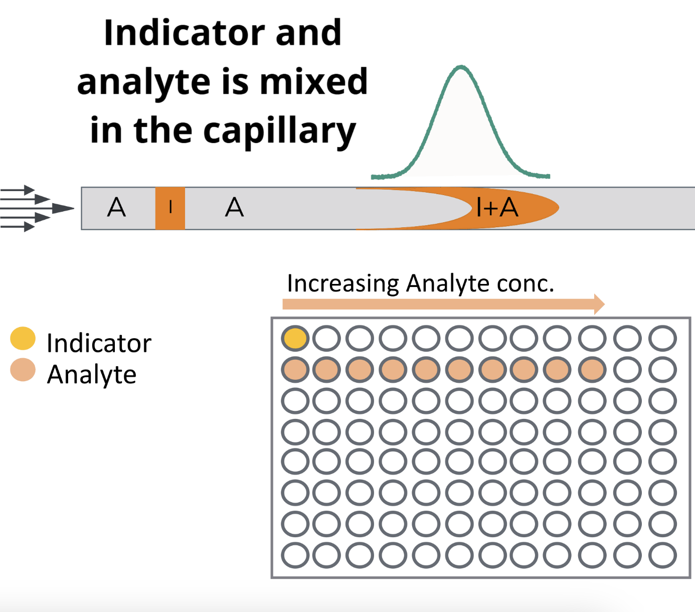
Capillary mix (Capmix) is where the indicator and the analyte mix inside the capillary. In a Capmix assay there is only a single indicator position and a titration of analytes.

The capillary is filled with an analyte and the indicator is introduced with no analyte mixed in before the assay. When the indicator plug is mobilised with the analyte, the indicator is diluted into the analyte.

In a Capmix assay the mixing and reaction time is controlled by the mobilisation pressure. Doubling the pressure will result in the sample arriving at the detector in half the time, also cutting the reaction time in half.

Recommended sample requirements

• Minimum 10 µL indicator total
• 50 µL analyte per data point for a triplicate
• 100 µL of analyte stock at 20 fold the expected K_D

Advantages

• Only 40 nL of indicator used per data point (1.4 µL sample for a 12 point titration in triplicate)
• Very little sample prep
• Exactly the same amount of indicator in each data point
• Controlled and known reaction time

Disadvantages

• Slow kinetics will give a skewed K_D

Recommended when assaying

• In-solution kinetics (required), see How to measure binding kinetics in solution?
• Assays where the indicator is precious (e.g. membrane proteins)
• Assays relying on very small changes in Binding Related Intensity Change (BRIC)

Capillary dissociation

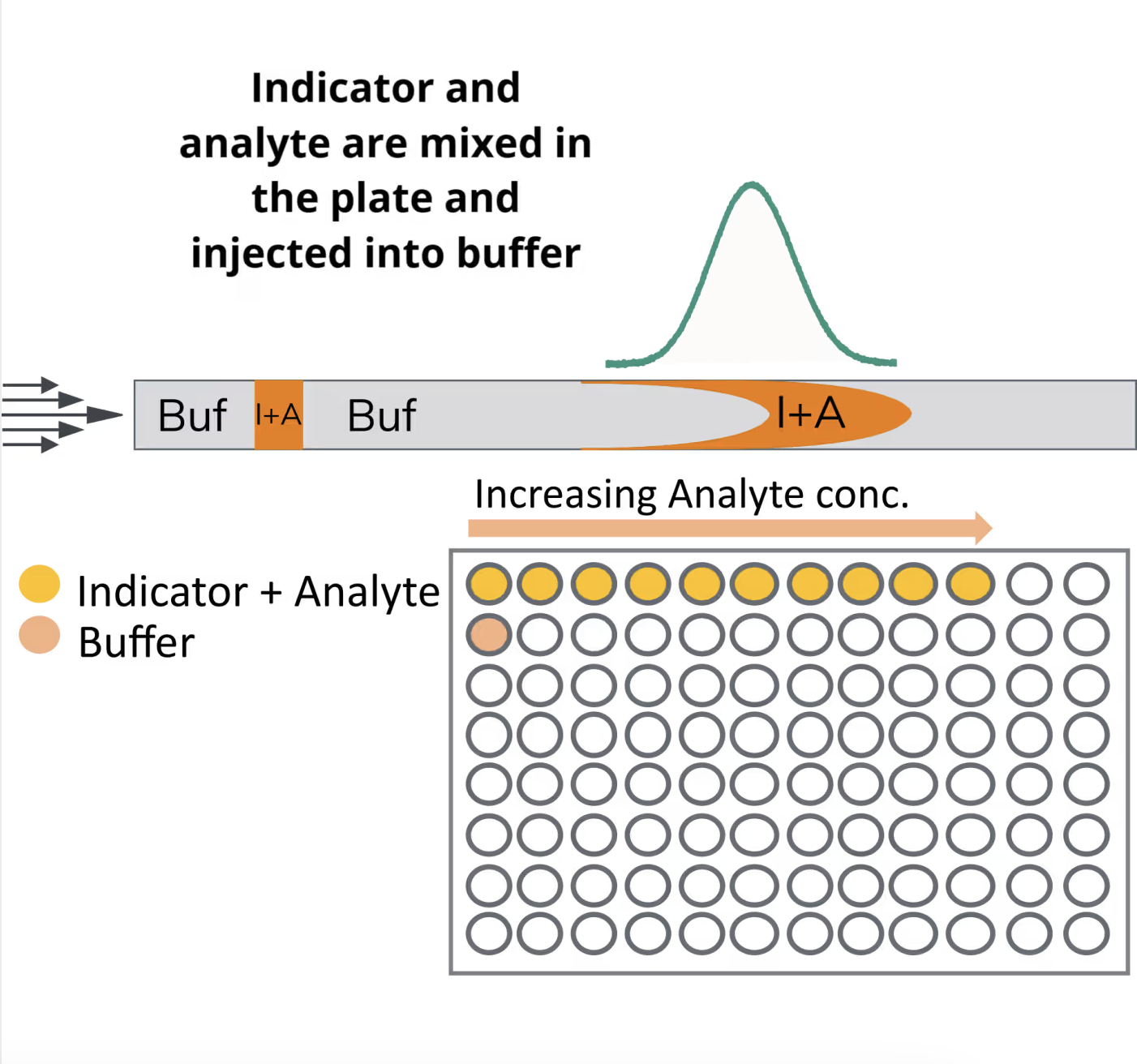
Capillary dissociation (CapDis) is an approach in which the analyte and indicator are mixed before being put in the autosampler and injected into buffer. In a CapDis assay there is a series of indicators with increasing concentration of analyte. These are then injected into buffer. This causes a dilution of the sample, potentially dissociating a given complex.

In a CapDis assay the time to reach the detector is controlled by the mobilisation pressure. Doubling the pressure will result in the sample arriving at the detector in half the time, also cutting the potential dissociation time in half.

Sample requirements

• Minimum 10 µL indicator + analyte per data point
• A couple of µL buffer
• Analyte stock at 20 fold the expected K_D

Advantages

• Very low use of precious analytes
• Very little sample prep

Disadvantages

• Fast dissociation kinetics may skew the K_D

Use this approach for/when:

• Large scale binding screen
• Indicator and analyte are extremely sticky, see How do you stop protein sticking to surfaces?
• Analyte is precious

Rapid K_D

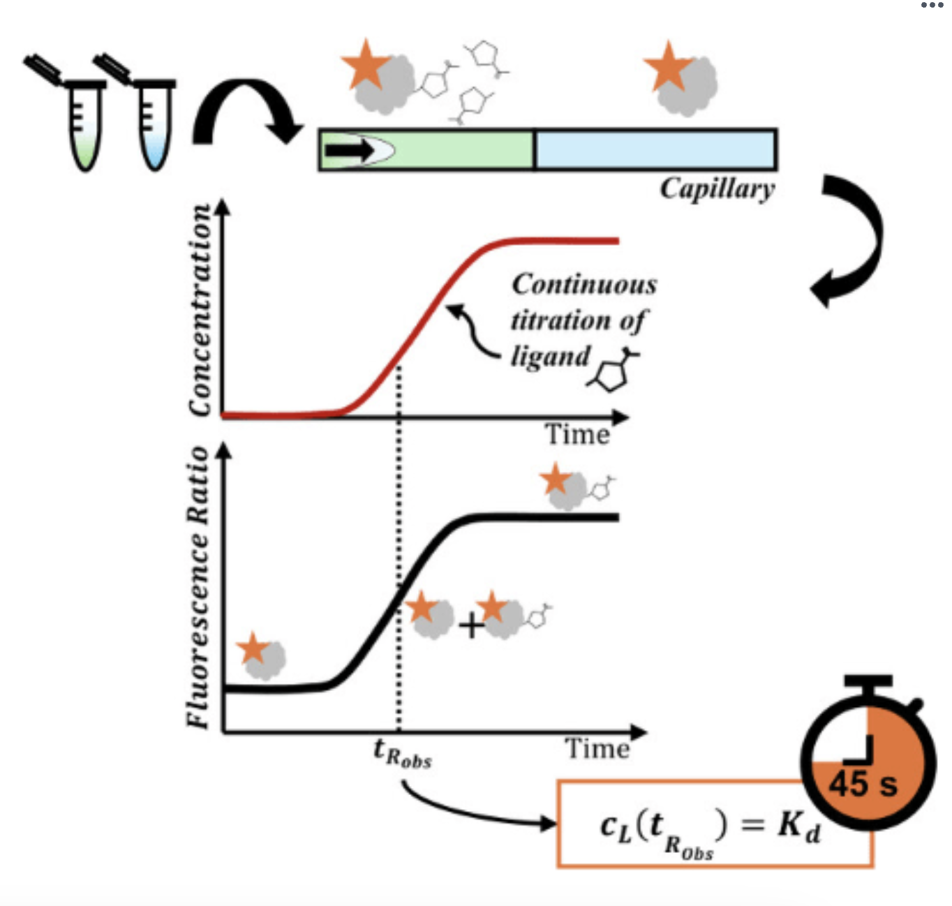
Continuous Titration Based Spectral Related Intensity Change (cSPRING), affectionately nicknamed fast or rapid K_D. The analyte and the indicator are mixed as a gradient during the run, allowing K_D determination in minutes. A cSPRING assay can be used to determine the K_D between a biomolecule labelled with an environment-sensitive fluorophore and a given interaction partner in less than a minute.

In a cSPRING experiment only a single indicator mixed with a saturating concentration of analyte and a single indicator without any analyte is required.

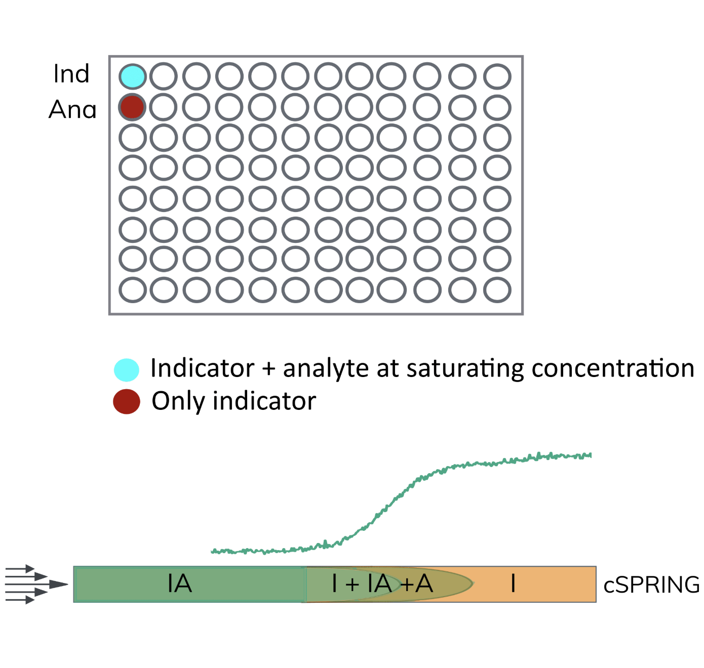
The capillary is filled with the free indicator (I), and the indicator mixed with the analyte is then mobilised through the capillary. This causes a concentration gradient of analyte to occur between the indicator phase and the indicator + analyte phase. The indicator concentration remains constant.

In a typical cSPRING experiment, the initial baseline is the signal from the unbound indicator and the final baseline the signal from the completely bound indicator. The change in signal between the two baselines represents the change in signal going from free to bound in the analyte gradient. Initially the concentration of analyte is 0, and as the gradient interface passes the detector it increases linearly until the maximum concentration is reached. The concentration of the indicator does not change during the experiment.

The data analysis is handled by the Fida software. For details on the fitting functions, see the publication Continuous Titration Based Method for Rapid In-Solution Analysis of Non-Covalent Interactions by Philipp Willmer and colleagues (Chemistry Methods, 2025, DOI: 10.1002/cmtd.202400059).

What parameters do you get?

• K_D, the apparent dissociation constant. The accuracy of the K_D depends on the interaction kinetics of the system and the mobilisation pressure.
• The hydrodynamic radius of the analyte. The experiment is set up like a front-loaded Taylor dispersion analysis (TDA) experiment with regard to the analyte. Therefore, the shape of the gradient between the two baselines contains information about the size of the analyte.

Advantages

• K_D measured in less than a minute
• Only 2 samples per K_D, very little sample prep
• Size information on your analyte

Disadvantages

• Sensitive to buffer changes: the buffers between the bound and free form must match
• No information on the size of the indicator or complex
• Requires relatively fast kinetics

Sample requirements

• Indicator concentration below the expected K_D
• Analyte concentration at 20 fold the expected K_D
• 10 µL of free indicator
• 10 µL of indicator + analyte

Capflex & TDIPS

Capflex and TDIPS are complex FIDA analysis formats used to study biomolecules undergoing liquid-liquid phase separation (LLPS). Liquid-liquid phase separation is biomolecules reversibly condensing into a liquid, concentrated, low water dense phase and a liquid, dilute, high water content phase.

• Some proteins can undergo a phase transition into a concentrated condensed phase under certain conditions
• This is a critical part of the function and regulation of many proteins
• Protein LLPS is involved in the formation of membrane-less organelles such as stress granules, the nucleolus and centrosomes, and is a vital process to life
• Misregulation of this process is at the heart of many neurodegenerative diseases

There is a minimum concentration of biomolecule required for LLPS to occur, referred to as the critical concentration or dilute phase concentration. More on LLPS is on the biomolecular condensates page.

Capflex

Capillary flow experiment (Capflex) is a method to study biomolecules undergoing LLPS. In a Capflex assay we quantify:

• Dilute phase concentration
• Number of droplets (spikes)
• Spike intensity

If the LLPS has a biphasic phase diagram, the spike intensity is proportional to droplet size.

In this method, phase-separated samples are incubated in a temperature-controlled tray and subsequently injected into a temperature-controlled capillary. As the injected sample traverses the capillary, a detector captures the signal. Each passing droplet within the capillary elicits a spike in the signal, while the baseline between spikes corresponds to the concentration of the dilute phase. This method can also be used to induce LLPS inside the capillary, by keeping the capillary temperature below the critical temperature and the temperature of the autosampler above the critical temperature.

When there is no LLPS occurring, the data looks like a sigmoidal curve with the top baseline corresponding to the protein concentration. When the sample has undergone LLPS, there are spikes appearing before the final baseline is reached as well as on the top baseline. The top baseline corresponds to the light phase concentration, the spikes to the number of droplets, and in some cases the spike intensity corresponds to droplet size. To get the dilute phase concentration, a standard curve of known protein concentration with no LLPS occurring needs to be done to calibrate the concentration.

Sample requirements

• The molecule of interest must be fluorescent, ideally labelled with a fluorophore insensitive to the local environment (e.g. ALC480 or GFP)
• Minimum volume is 10 µL, as a measurement will consume about 8 µL; this can be reduced using thinner capillaries
• The average viscosity of the solution should be less than 40 cP

Advantages

• Measure dilute phase concentration, droplet count and relative droplet size in one experiment
• No buffer restrictions
• Low sample consumption
• Assay can be performed so it accounts for ageing

Disadvantages

• Labelled samples required (only at trace concentrations)
• Uses more sample than TDIPS

The original method paper is the publication Capillary flow experiments for thermodynamic and kinetic characterization of protein liquid-liquid phase separation (Nature Communications, 2021).

TDIPS

Taylor dispersion induced phase separation (TDIPS) is a label-free screening method for LLPS that can also be used to generate phase diagrams and dose response curves, using nL of sample per data point. It works by inducing LLPS inside the capillary without any labels, thus having complete control of reaction times.

In TDIPS you store the sample of interest in the sample holder in a condition where it does not phase separate (e.g. freezer storage buffer). The capillary is filled with a condition in which LLPS can occur, then a plug of your sample is injected and mobilised with the LLPS inducing buffer. As a biomolecule has a much slower diffusion rate than the storage buffer molecules, the molecule of interest is dispersed into the LLPS buffer, causing LLPS to occur, while the original condition remains in the centre of the plug. As droplets in turn have a much slower diffusion than a protein, the larger droplets are flow focused and outrun the sample plug, and potentially dissolve, as the local concentration of biomolecule will be lower than the critical concentration. The method can also be run in a plug sandwich format, allowing for dose response and screening of precious LLPS modifying compounds.

If no LLPS occurs, the data looks like a standard Taylorgram. The Fida software can count the spikes in the data, which is the primary readout of the experiment. For analysis of the integral and decrease in fluorescence, there is a published script available from the authors.

Sample requirements

• Molecule of interest must be fluorescent at a wavelength suitable for the Fida detectors
• 10 µL of molecule of interest in a buffer condition where it does not undergo LLPS
• Buffer at least 50 µL, ideally more

Advantages

• Using TDIPS, phase diagrams can be recorded label-free with µL of sample
• TDIPS can screen for LLPS with nL sample use of both compound and biomolecule
• The data is very information rich, testing both for reversibility and the amount of material that has phase separated
• TDIPS can be done label-free and is in solution
• Anyone with a Fida instrument can get started immediately

Disadvantages

• The method cannot be used as a standalone; follow-up with microscopy or Capflex is required
• Not suitable for LLPS modifying compounds that are fluorescent at the same wavelength as the chosen assay wavelength

The original method paper is Taylor Dispersion-Induced Phase Separation for the Efficient Characterisation of Protein Condensate Formation.

Non-Taylor condition assays (MTIS)

Molecules can be analysed under non-Taylor conditions, also known as microfluidic transient incomplete separation (MTIS). The pressure is set so only your protein of interest is in Taylor's condition. An MTIS experiment is a Premix experiment where the mobilisation pressure is set at a level where everything larger than your molecule of interest is outside Taylor's conditions and is flow focused. As the sample of interest is mobilised, molecules larger than the size determined by the set pressure are flow focused and partially separated from the molecule of interest.

Fitting the data yields the amount of material outside Taylor's condition and the amount of molecule of interest still in Taylor's condition. For example, MTIS has been used to study the depolymerisation of an amyloid fibril, in the publication Thermodynamic characterization of amyloid polymorphism by microfluidic transient incomplete separation (Chemical Science, 2024).

Before an MTIS experiment, you should know the size of the monomer. In the Fida software, click Utilities and select Experimental evaluation. This brings up the experimental evaluation window, where you can test whether your experimental parameters are in Taylor's condition. For example, for a monomer size of 5.93 nm and a running pressure of 1200 mbar, Tau is too low and Taylor's condition is not met. The software determines that the maximum running pressure is 893 mbar. At this pressure, all species bigger than 6 nm will be flow focused.

MTIS data analysis is not part of the Fida software package, but details on the fitting can be found in the original method paper.

What can it be used for?

• Amyloid fibril stability determination
• Rapid binding confirmation screens
• Biomolecules binding to large particles for K_D determination

Frequently asked questions

Which FIDA assay format should I use to study an interaction at equilibrium?

Premix, where the indicator and analyte are mixed before the run and are at equilibrium.

Which format should I use when the indicator is precious?

Capmix, which uses only 40 nL of indicator per data point.

Which format should I use when the analyte is precious?

CapDis, which uses very little analyte.

Is a Premix needed for in-solution kinetics?

Yes. In-solution kinetics needs both a Premix, for the equilibrium K_D, and a Capmix.

Related resources

Want to see LLPS measured on a Fida instrument? The poster Rapid characterization of LLPS with FIDA shows dilute phase concentration, droplet formation kinetics, amyloid fibril maturation and modulator binding affinity measured with FIDA.

New to binding assays? How to perform a binding affinity assay? walks through a binding measurement, Which binding model should you use to fit FIDA affinity data? explains the binding models used to fit the data, What is K_D (dissociation constant)? explains the affinity each format reports, and How much sample do you need to measure binding affinity and size? covers sample consumption. The full Assay formats course is on the Fidabio Learning Hub: register for the Fidabio Learning Hub.